Session 8: ODE stability; stiff system
Date: 11/06/2017, Monday
In [1]:
format compact
ODE Stability
Problem statement
Consider a simple ODE
where \(a\) is a positive real number.
It can be solved analytically:
So the analytical solution decays exponentially. A numerical solution is allowed to have some error, but it should also be decaying. If the solution is instead growing, we say it is unstable.
Explicit scheme
Forward Eulerian scheme for this problem is
The iteration is given by
The solution at the k-th time step can be written out explicitly
We all know that when \(h\) gets smaller the numerical solution will converge to the true result. But here we are interested in relatively large \(h\), i.e. we wonder what’s the largest possible \(h\) we can use while still getting an OK result.
Here are the solutions with different \(h\).
In [2]:
%plot -s 400,300

% set parameters, can use different value
a = 1;
y0 = 1;
tspan = 10;

% build function
f_true = @(t) y0*exp(-a*t); % true answer
f_forward = @(k,h) (1-h*a).^k * y0; % forward Euler solution

% plot true result
t_ar = linspace(0, tspan); % for plotting
y_true = f_true(t_ar);
plot(t_ar, y_true)
hold on

% plot Forward Euler solution
for h=[2.5, 1.5, 0.5] % try different step size
    kmax = round(tspan/h);
    k_ar = 0:kmax;
    t_ar = k_ar*h;

    % we are not doing Forward Euler iteration here
    % since the expression is known, we can directly
    % get the entire time series
    y_forward = f_forward(k_ar, h);

    plot(t_ar, y_forward, '-o')
end

% tweak details
ylim([-1,1]);
xlabel('t');ylabel('y');
legend('true solution', 'h=2.5', 'h=1.5', 'h=0.5' , 'Location', 'Best')
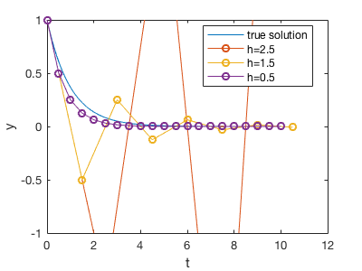
There all 3 typical regimes, determined by the magnitude of \([1-ha]\) inside the expression \(y_k= (1-ha)^ky_0\).
- Small \(h\): \(0 \le [1-ha] < 1\)
In this case, \((1-ha)^k\) will decay with \(k\) and always be positve.
We can solve for the range of \(h\):
This corresponds to h=0.5 in the above figure.
- Medium \(h\): \(-1 \le [1-ha] < 0\)
In this case, the absolute value of \((1-ha)^k\) will decay with \(k\), but it oscillates between negative and postive. This is not desirable, but not that bad, as our solution doesn’t blow up.
We can solve for the range of \(h\):
This corresponds to h=1.5 in the above figure.
- Large \(h\): \([1-ha] < -1\)
In this case, the absolute value of \((1-ha)^k\) will increase with \(k\). That’s the worst case because the true solution will be decaying, but our numerical solution insteads gives exponential growth. Here our numerical scheme is totally wrong, not just inaccurate.
We can solve for the range of \(h\):
This corresponds to h=2.5 in the above figure.
The take-away is, to obtain a stable solution, the time step size \(h\) needs to be small enough. The time step requirement depends on \(a\), i.e. how fast the system is changing. If \(a\) is large, i.e. the system is changing rapidly, then \(h\) has to be small enough (\(h<1/a\) or \(h<2/a\), depends on what your want) to capture this fast change.
Implicit scheme
But sometimes we really want to use a large step size. For example, we might only care about the steady state where \(t\) is very large, so we would like to quickly jump to the steady state with very few number of iterations. Implicit method allows us to use a large time step while still keep the solution stable.
Backward Eulerian scheme for this problem is
In general, the right hand-side would be some function \(f(y_{k+1})\), and we need to solve a nonlinear equation to obtain \(y_{k+1}\). This is why this method is called implicit. But in this problem here we happen to have a linear function, so we can still write out the iteration explicitly.
The solution at the k-th time step can be written as
Here are the solutions with different \(h\).
In [3]:
%plot -s 400,300

% set parameters, can use different value
a = 1;
y0 = 1;
tspan = 10;

% build function
f_true = @(t) y0*exp(-a*t); % true answer
f_backward = @(k,h) (1+h*a).^(-k) * y0; % backward Euler solution

% plot true result
t_ar = linspace(0, tspan); % for plotting
y_true = f_true(t_ar);
plot(t_ar, y_true)
hold on

% plot Forward Euler solution
for h=[2.5, 1.5, 0.5] % try different step size
    kmax = round(tspan/h);
    k_ar = 0:kmax;
    t_ar = k_ar*h;

    % we are not doing Forward Euler iteration here
    % since the expression is known, we can directly
    % get the entire time series
    y_backward = f_backward(k_ar, h);

    plot(t_ar, y_backward, '-o')
end

% tweak details
ylim([-0.2,1]);
xlabel('t');ylabel('y');
legend('true solution', 'h=2.5', 'h=1.5', 'h=0.5' , 'Location', 'Best')
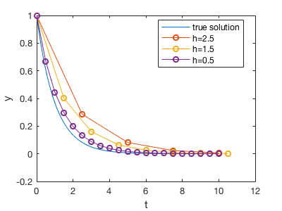
Since \(\frac{1}{1+ha}\) is always smaller than 1 for any positive \(h\) and postive \(a\), \(y_k= \frac{y_k}{(1+ha)^k}\) will always decay. So we don’t have the instability problem as in the explicit method. A large \(h\) simply gives inaccurate results, but not terribly wrong results.
According to no free lunch theorm, implicit methods must have some additional costs (half joking. that’s another theorm). The cost for an implicit method is solving a nonlinear system. In general we will have \(f(y, t)\) on the right-hand side of the ODE, not simply \(-ay\).
General form
Using \(-ay\) on the right-hand side allows a simple analysis, but the idea of ODE stability/instability applies to general ODEs. For example considering a system like
You can use the typical magnitude of \(f(t)\) as the “\(a\)” in the previous analysis.
Even for
You can consider the typical magnitude of \(yf(t)\)
Stiff system
Consider an ODE system
Using an explicit method, the time step requirement for the first equation is \(h<1/a_1\), while the requirement for the second one is \(h<1/a_2\). If \(a_1 >> a_2\), we have to use a quite small \(h\) to accomodate the first requirement, but that’s an overkill for the second equation. You will be using too many unnecessary time steps to solve \(y_2\)
We can define the stiff ratio \(r=\frac{a_1}{a_2}\). A system is very stiff if \(r\) is very large. With explicit methods you often need an unnecessarily large amount of time steps to ensure stability. Implicit methods are particularly useful for a stiff system because it has no instability problem.
You might want to solve two equations separately so we can use a larger time step for the second equation to save computing power. But it’s not that easy because in real examples the two equations are often intertwined: