Lecture 5: Random Numbers & Complex Numbers

Date: 09/14/2017, Thursday

format compact

Built-in random number generator

rand returns a random number between [0,1] (uniform distribution).

rand

ans =
    0.8147

rand(N) returns a \(N \times N\) random matrix. You can always type doc rand or help rand to see the detailed usage.

rand(5)

ans =
    0.9058    0.2785    0.9706    0.4218    0.0357
    0.1270    0.5469    0.9572    0.9157    0.8491
    0.9134    0.9575    0.4854    0.7922    0.9340
    0.6324    0.9649    0.8003    0.9595    0.6787
    0.0975    0.1576    0.1419    0.6557    0.7577

randi(N) returns an integer between 1 and N.

randi(100)

ans =
    75

randn uses normal distribution, instead of uniform distribution.

randn(5)

ans =
   -0.3034   -1.0689   -0.7549    0.3192    0.6277
    0.2939   -0.8095    1.3703    0.3129    1.0933
   -0.7873   -2.9443   -1.7115   -0.8649    1.1093
    0.8884    1.4384   -0.1022   -0.0301   -0.8637
   -1.1471    0.3252   -0.2414   -0.1649    0.0774

Complex numbers

Complex number basics

A real number (double-precision) takes 8 Bytes (64 bits). A complex number is a pair of numbers so simply takes 16 Bytes (128 bits)

x = 3;
y = 4;
z = x+i*y;

whos

  Name      Size            Bytes  Class     Attributes

  ans       5x5               200  double
  x         1x1                 8  double
  y         1x1                 8  double
  z         1x1                16  double    complex

Take conjugate of a complex number:

conj(z)

ans =
   3.0000 - 4.0000i

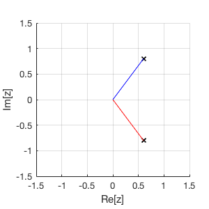
Show the number on the complex plane

%plot --size 300,300
hold on
complex_number_plot_fn(conj(z)/5,'r') % complex_number_plot_fn is available on canvas.
complex_number_plot_fn(z/5,'b')

3 equivalent ways to compute \(|z|\)

abs(z)

ans =
     5

sqrt(dot(z,z))

ans =
     5

norm(z)

ans =
     5

The angle of z in degree:

angle(z) / pi * 180.0

ans =
   53.1301

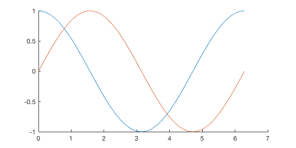
Euler’s Formula

\[e^{i\theta} = \cos(\theta) + i\sin(\theta)\]

Verify that MATLAB understands \(e^{i\theta}\)

theta = linspace(0, 2*pi, 1e4);
z = exp(i*theta); % now z is an array, not a scalar as defined in the previou section.

%plot --size 600,300
hold on
plot(theta,real(z))
plot(theta,imag(z))

Mandelbrot set

Iteration with a single parameter

c = rand-0.5 + i*(rand-0.5);

T = 50;
z_arr = zeros(T,1); % to hold the entire time series

z = 0; % initial value
z_arr(1) = z;

for t=2:T
    z = z^2+c;
    z_arr(t) = z;
end

hold on
plot(real(z_arr))
plot(imag(z_arr))

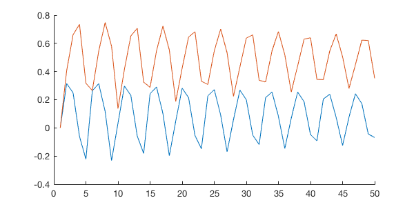
Run this code repeatedly, you will see sometimes \(z\) will blow up, sometime not, according to the initial value of \(c\). Thus we want to figure out what values of \(c\) will make \(z\) blow up.

Iteration with the entire paremeter space

We want to construct a 2D array containing all possible values of \(c\) on the complex plane.

Let’s make 1D grids first.

nx = 100;
xm = 1.75;
x = linspace(-xm, xm, nx);
y = linspace(-xm, xm, nx);

size(x), size(y)

ans =
     1   100
ans =
     1   100

convert 1D grid to 2D grid.

[Cr, Ci] = meshgrid(x,y);

size(Cr), size(Ci)

ans =
   100   100
ans =
   100   100

C = Cr + i*Ci; % now C spans over the complex plane

size(C)

ans =
   100   100

Run the iteration for every value of C

T = 50;

Z_final = zeros(nx,nx); % to hold last value of z, at all possible points.

for ix = 1:nx
for iy = 1:nx % we also have nx points in the y-direction

    % get the value of c at current point.
    % note that MATLAB is case-sensitive
    c = C(ix,iy);

    z = 0; % initial value, doesn't matter too much
    for t=2:T
        z = z^2+c;
    end
    Z_final(ix,iy) = z; % save the last value of z

end
end

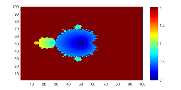
Here’s one way to visualize the result.

pcolor(abs(Z_final)); % plot the magnitude of z

shading flat; % hide grids
colormap jet; % change colormap
colorbar; % show colorbar

% The default color range is min(z)~max(z),
% but max(z) is almost Inf so we make the range smaller
caxis([0,2]);