Session 9: Partial differential equation

Date: 11/13/2017, Monday

format compact

I assume you’ve learnt very little about PDEs in basic math class, so I would first talk about PDEs from a programmer’s perpesctive and come to the math when necessary.

PDE from a programmer’s view: You already know that ODE is the evolution of a single value. From the current alue \(y_t\) you can solve for the next value \(y_{t+1}\). PDE is the evolution of an array. From the current array \((x_1,x_2,...,x_m)_t\) you can solve for the array at the next time step \((x_1,x_2,...,x_m)_{t+1}\). Typically, the array represents some physical field in the space, like 1D temperature distribution.

Naive advection “solver”

Consider a spatial domain \(x \in [0,1]\). We discretize it by 11 points including the boundary.

x = linspace(0,1,11)
nx = length(x)

x =
  Columns 1 through 7
         0    0.1000    0.2000    0.3000    0.4000    0.5000    0.6000
  Columns 8 through 11
    0.7000    0.8000    0.9000    1.0000
nx =
    11

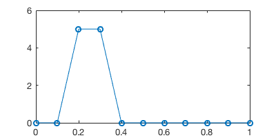
The initial physical field (e.g. the concentration of some chemicals) is 5.0 for \(x \in [0.2,0.3]\) and zero elsewhere. Let’s create the initial condition array.

u0 = zeros(1,nx); % zero by default
u0(3:4) = 5.0; % non-zero between 0.2~0.3

%plot -s 400,200
plot(x, u0, '-o')
ylim([0,6]);

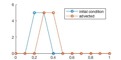
Say the chemical is blew by the wind towards the right. At the next time step the field is shifted rightward by 1 grid point.

To represent the solution at the next time step, we could create a new array u_next and set u_next(4:5) = 5.0, based on our knowledge that u0(3:4) = 5.0. However, we want to write code that works for any initiatial condition, so the code would look like:

% initialization
u = u0;
u_next = zeros(1,nx); % initialize to 0

% shift rightward
u_next(2:end) = u(1:end-1);

% just plotting
hold on
plot(x, u, '-o')
plot(x, u_next, '-o')
ylim([0,6]);
legend('initial condition', 'advected')

Space-time diagram

We can keep shifting the field and record the solution at 5 time steps.

u = u0; % reset solution
u_next = zeros(1,nx); % reset solution
u_ts = zeros(5,nx); % to record the entire time series

u_ts(1,:) = u; % record initial condition

for t=2:5
    u_next(2:end) = u(1:end-1); % shift rightward
    u = u_next; % swap arrays for the next iteration
    u_ts(t,:) = u; % record current step
end

% just plotting
hold on
for t=1:5
    plot(x, u_ts(t, :), '-o')
end
ylim([0,6]);
legend('t=0', 't=1', 't=2', 't=3', 't=4')

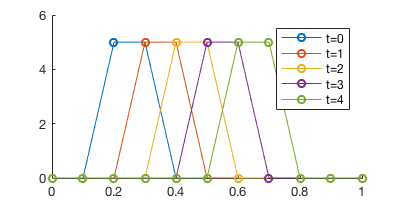
The plot looks quite convoluted with multiple time steps… A better way to visualize it is to plot the time series in a 2D x-t plain.

contourf(x,0:4,u_ts)
colorbar()
xlabel('x');ylabel('time')
title("space-time diagram")

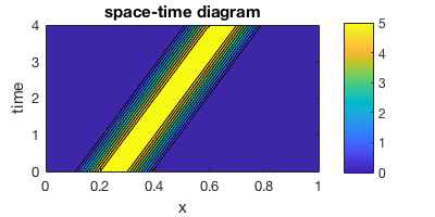
Here we can clearly see the “chemical field” is moving rightward through time.

Advection equation

We call this rightward shift an advection process. Just like the diffusion process introduced in the class, advection happens everywhere in the physical world. In general, the physical field won’t be shifted by exact one grid point. Instead, we can have arbitrary wind speed, changing with space and time. To represent this general advection process, we can write a partial differential equation:

Advection equation with initial condition \(u_0(x)\)

\[\frac{\partial u}{\partial t}+c\frac{\partial u}{\partial x} = 0, \ \ u(x,0) = u_0(x)\]

This means a phyical field \(u(x,t)\) is advected by wind speed \(c\). In general, the wind speed \(c(x,t)\) can change with space and time. But if \(c\) is a constant, then the analytical solution is

\[u(x,t) = u_0(x-ct)\]

You can verify this solution by bringing it back to the PDE.

We ask, “what’s the chemical concentration at a spatial point \(x=x_j\), when \(t=t_n\)“? According to the solution, the answer is, “it is the same as the concentration at \(x=x_j-ct_n\) when \(t=0\)“. This is physically intuitive. The chemical originally at \(x=x_j-ct_n\) was traveling rightward at speed \(c\), so after time period \(t_n\) it would reach \(x=x_j\). Thus in order to find the concentration at \(x=x_j\) right now, what we can do is going backward in time to find where does the current chemical come from.

This solution-finding process means going downward&leftward along the contour line in space-time diagram shown before.

Numerical approximation to advection equation

In practice, \(c\) is often not a constant, so we can’t easily find an anlytical solution and must rely on numerical methods.

Use first-order finite difference approximation for both \(\frac{\partial u}{\partial t}\) and \(\frac{\partial u}{\partial x}\):

\[\frac{u_j^{n+1}-u_j^n}{\Delta t} + c\frac{u_j^{n}-u_{j-1}^n}{\Delta x} = 0\]

Let \(\alpha=\frac{c \Delta t}{\Delta x}\), the iteration can be written as

\begin{align} u_j^{n+1} &= u_j^n - \alpha(u_j^{n}-u_{j-1}^n) \\ &= (1-\alpha)u_j^n + \alpha u_{j-1}^n \end{align}

Note that, to approximate \(\frac{\partial u}{\partial x}\), we use \(\frac{u_j-u_{j-1}}{\Delta x}\) instead of \(\frac{u_{j+1}-u_{j}}{\Delta x}\). There’s an important physical reason for that. Here we assume \(c\) is positive (rightward wind), so the chemical should come from the leftside (\(u_{j-1}\)), not the rightside (\(u_{j+1}\)).

Finally, notice that when \(\alpha=1\) we effectively get the previous naive “shifting” scheme.

One step integration

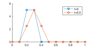
We set \(c=0.1\) and \(\Delta t=0.5\), so after one time step the chemical would be advected by half grid point (recall that our grid interval is 0.1).

Coding up the scheme is straightforward. The major difference from ODE solving is your are updating an array, not a single scalar.

% set parameters
c = 0.1; % wind velocity
dx = x(2)-x(1)
dt = 0.5;
alpha = c*dt/dx

% initialization
u = u0;
u_next = zeros(1,nx);

% one-step PDE integration
for j=2:nx
    u_next(j) = (1-alpha)*u(j) + alpha*u(j-1);
    % think about what to do for j=1?
    % we will talk about boundaries later
end

% plotting
hold on
plot(x, u, '-o')
plot(x, u_next, '-o')
ylim([0,6]);
legend('t=0', 't=0.5')

dx =
    0.1000
alpha =
    0.5000

Multiple steps

To integrate for multiple steps, we just add another loop for time.

% re-initialize
u = u0;
u_next = zeros(1,nx);

% PDE integration for 2 time steps
for t = 1:2 % loop for time
    for j=2:nx % loop for space
        u_next(j) = (1-alpha)*u(j) + alpha*u(j-1);
    end
    u = u_next;
end

% plotting
hold on
plot(x, u0, '-o')
plot(x, u, '-o')
ylim([0,6]);
legend('t=0', 't=1')

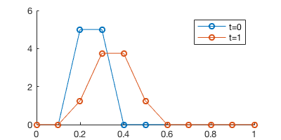
We got a pretty huge error here. After \(t=0.5 \times 2=1\), the solution should just be shifted by one grid point, like in the previous naive PDE “solver”. Here the center of the chemical field seems alright (changed from 0.25 to 0.35), but the chemical gets diffused pretty badly. That’s due to the numerical error of the first-order scheme.

Does decreasing time step size help?

In ODE solving, we can always reduce time step size to improve accuracy. Does the same trick help here?

c = 0.1;
dx = x(2)-x(1);
dt = 0.1; % use a much smaller time step
nt = round(1/dt) % calculate the number of time steps needed
alpha = c*dt/dx


% === exactly the same as before ===
u = u0;
u_next = zeros(1,nx);

for t = 1:nt
    for j=2:nx
        u_next(j) = (1-alpha)*u(j) + alpha*u(j-1);
    end
    u = u_next;
end

hold on
plot(x, u0, '-o')
plot(x, u, '-o')
ylim([0,6]);
legend('t=0', 't=1')

nt =
    10
alpha =
    0.1000

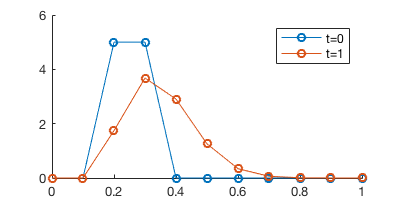
Oops, there is no improvement.

That’s because we have both time discretization error \(O(\Delta t)\) spatial discretization error \(O(\Delta x)\) in PDE solving. The total error for our scheme is \(O(\Delta t)+O(\Delta x)\). Simply decreasing the time step size is not enough. To improve accuracy you also need to increase the number of spatial grid points (nx).

Another way to improve accuracy is to use high-order scheme. But designing high-order advection scheme is quite challenging. You can find tons of papers by searching something like “high-order advection scheme”.

Boundary condition

So far we’ve ignored the boundary condition. Because the field is shifting rightward, the leftmost grid point is able to receive information from the “outside”. Think about a pipe where new chemicals keep coming in from the left.

Our previous specification of the advection equation is not complete. The complete version is:

Advection equation with initial condition \(u_0(x)\) and left boundary condition \(u_{left}(t)\)

\[\begin{split}\frac{\partial u}{\partial t}+c\frac{\partial u}{\partial x} = 0 \\ u(x,0) = u_0(x) \\ u(0,t) = u_{left}(t)\end{split}\]

Here we assume \(u_{left}(t)=5\). In the code, you just need to add one line.

c = 0.1;
dx = x(2)-x(1);
dt = 0.1;
nt = round(1/dt);
alpha = c*dt/dx;

u = u0;
u_next = zeros(1,nx);

for t = 1:nt

    u_next(1) = 5.0; % the only change!!
    for j=2:nx
        u_next(j) = (1-alpha)*u(j) + alpha*u(j-1);
    end
    u = u_next;
end

hold on
plot(x, u0, '-o')
plot(x, u, '-o')
ylim([0,6]);
legend('t=0', 't=1')

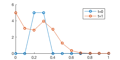
We can now see new chemicals are “injected” from the left side.

Stability

Numerical experiment

PDE solvers also have stability requirements, just like ODE solvers. The general idea is the time step needs to be small enough, compared to the spatial step. This holds for advection, diffusion, wave and various forms of PDEs, although the exact formula for time step requirement can be different depending on the problem.

Here we use a much larger time step to see what happens.

c = 0.1;
dx = x(2)-x(1);
dt = 2; % a much larger time step
alpha = c*dt/dx

u = u0;
u_next = zeros(1,nx);

for t = 1:10
    for j=2:nx
        u_next(j) = (1-alpha)*u(j) + alpha*u(j-1);
    end
    u = u_next;

    if t == 1 % record the first time step
        u1 = u;
    end
end

hold on
plot(x, u0, '-o')
plot(x, u1, '-o')
plot(x, u, '--')
ylim([-40,40]);
legend('initial', 't=2', 't=20')

alpha =
     2

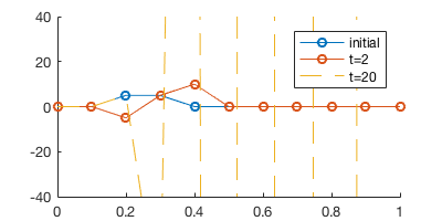
The simulation blows very quickly.

Intuitive explanation

In the previous experiment we have \(\alpha=2\), so one of the coeffcients in the formula becomes negative:

\[u_j^{n+1} = (1-\alpha)u_j^n + \alpha u_{j-1}^n = (-1)\times u_j^n + 2\times u_{j-1}^n\]

Negative coefficients are meaningless here, because a grid point \(x_j\) shouldn’t get “negative contribution” from a nearby grid point \(x_{j-1}\). It makes no sense to advect “negative density” or “negative concentration”.

To keep both coefficients (\(\alpha\) and \(1-\alpha\)) postive, we require \(0 \le \alpha \le 1\). Recall \(\alpha = \frac{c \Delta t}{\Delta x}\), so we essentially require the time step to be small.

This is just an intuitive explanation. To rigorously derive the stability requirement, you would need some heavy math as shown below.

Stability analysis (theoretical)

The time step requirement can be derived by von Neumann Stability Analysis (also see PDE_solving.pdf on canvas).

The idea is we want to know how does the magnitude of \(u_j^{n}\) change with time, under the iteration (first-order advection scheme for example):

\[u_j^{n+1} = (1-\alpha)u_j^n + \alpha u_{j-1}^n\]

It is troublesome to track the entire array \([u_1^{n},u_2^{n},...,u_m^{n}]\). Instead we want a single value to represent the magnitude of the array. The general idea is to perform Fourier expansion on the spatial field \(u(x)\). From Fourier analysis we know any 1D field can viewed as the sum of waves of different wavelength:

\[u(x) = \sum_{k=-\infty}^{\infty} T_k e^{ikx}\]

Thus we can track how a single component, \(T_k e^{ikx}\), evolves with time. We omit the subscript \(k\) and add the time index \(n\), so the component at the n-th time step can be written as \(T(n) e^{ikx}\). The iteration for this component is

\[T(n+1)e^{ikx} = (1-\alpha)T(n) e^{ikx} + \alpha T(n) e^{ik(x-\Delta x)}\]

Divide both sides by \(e^{ikx}\)

\[T(n+1) = (1-\alpha)T(n) + \alpha T(n) e^{-ik\Delta x}\]

\[\frac{T(n+1)}{T(n)} = 1-\alpha + \alpha e^{-ik\Delta x}\]

Define amplification factor \(A=\frac{T(n+1)}{T(n)}\). We want \(|A| \le 1\) so the solution won’t blow up, just like what we did in the ODE stability analysis.

We thus require

\[|1-\alpha + \alpha e^{-ik\Delta x}| \le 1\]

So we’ve transformed the requirement on an array to the requirement on a scalar.

We want this inequality to be true for any \(k\). It will finally lead to a requirement for \(\alpha\), which is the same as the previous intuitive analysis that \(0 \le \alpha \le 1\). Fully working this out needs some math, see this post for example.

High-order PDE

The wave equation is a typical 2nd-order PDE

\[\frac{\partial^2 u}{\partial t^2} - c^2\frac{\partial^2 u}{\partial x^2} = 0\]

Compared to the advection equation, the major differences are

• The wave can go both rightward and leftward, at speed \(c\) or \(-c\).
• It needs both left and right boundary condition. Periodic boundary conditions are often used.
• It needs both 0th-order and 1st-order initial conditions, i.e. \(u(x,t)|_{t=0}\) and \(\frac{\partial u}{\partial t} |_{t=0}\). Otherwise you can’t start your intergration, because a 2nd-order time derivative means \(u^{n+1}\) would rely on both \(u^{n}\) and \(u^{n-1}\). 0th-order initial condition only gives you one time step, but you need two time steps to get started.