Session 7: Error convergence of numerical methods

Date: 10/30/2017, Monday

format compact

Error convergence of general numerical methods

Many numerical methods has a “step size” or “interval size” \(h\), no mattter numerical differentiation, numerical intergration or ODE solving. We denote \(f(h)\) as the numerical approximation to the exact answer \(f_{true}\). Note that \(f\) can be a derivate, an integral or an ODE solution.

In general, the numerical error gets smaller when \(h\) is reduced. We say a method has \(O(h^k)\) convergence if

\[f(h) - f_{true} = C \cdot h^k + C_1 \cdot h^{k+1} + ...\]

As \(h \rightarrow 0\), we will have \(f(h) \rightarrow f_{true}\). Higher-order methods (i.e. larger \(k\)) leads to faster convergence.

Error convergence of numerical differentiation

Consider \(f(x) = e^x\), we use finite difference to approximate \(g(x)=f'(x)=e^x\). We only consider \(x=1\) here.

f = @(x) exp(x); % the function we want to differentiate

x0 = 1; % only consider this point
g_true = exp(x0) % analytical solution

g_true =
    2.7183

We try both forward and center schemes, with different step sizes \(h\).

h_list = 0.01:0.01:0.1; % test different step size h
n = length(h_list);
g_forward = zeros(1,n); % to hold forward difference results
g_center = zeros(1,n); % to hold center difference results

for i = 1:n % loop over different step sizes
    h = h_list(i); % get step size

    % forward difference
    g_forward(i) = (f(x0+h) - f(x0))/h;

    % center difference
    g_center(i) = (f(x0+h) - f(x0-h))/(2*h);
end

The first element in g_forward is quite accurate, but the error grows as the step size \(h\) gets larger.

g_forward

g_forward =
  Columns 1 through 7
    2.7319    2.7456    2.7595    2.7734    2.7874    2.8015    2.8157
  Columns 8 through 10
    2.8300    2.8444    2.8588

Center difference scheme is much more accurate.

g_center

g_center =
  Columns 1 through 7
    2.7183    2.7185    2.7187    2.7190    2.7194    2.7199    2.7205
  Columns 8 through 10
    2.7212    2.7220    2.7228

Compute the absolute error of each scheme

error_forward = abs(g_forward - g_true)
error_center = abs(g_center - g_true)

error_forward =
  Columns 1 through 7
    0.0136    0.0274    0.0412    0.0551    0.0691    0.0832    0.0974
  Columns 8 through 10
    0.1117    0.1261    0.1406
error_center =
  Columns 1 through 7
    0.0000    0.0002    0.0004    0.0007    0.0011    0.0016    0.0022
  Columns 8 through 10
    0.0029    0.0037    0.0045

Make a \(h \leftrightarrow error\) plot.

%plot -s 600,200
subplot(121); plot(h_list, error_forward,'-o')
title('forward');xlabel('h');ylabel('error')
subplot(122); plot(h_list, error_center,'-o')
title('center');xlabel('h');ylabel('error')

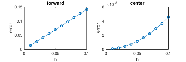
• Forward scheme gives a straight line because it is a first-order method and \(error(h) \approx C \cdot h\)
• Center scheme gives a parabola because it is a second-order method and \(error(h) \approx C \cdot h^2\)

Diagnosing the order of convergence

But by only looking at the \(error(h)\) plot, how can you know the curve is a parabola? Can’t it be a cubic \(C \cdot h^3\)?

Recall that in HW4 you were fitting a function \(R = bW^a\). To figure out the coefficients \(a\) and \(b\), you need to take the log. The same thing here.

If \(error = C \cdot h^k\), then

\[\log(error) = \log C + k \log h\]

The slope of the \(log(error) \leftrightarrow log(h)\) plot is \(k\), i.e. the order of the numerical method.

%plot -s 600,200
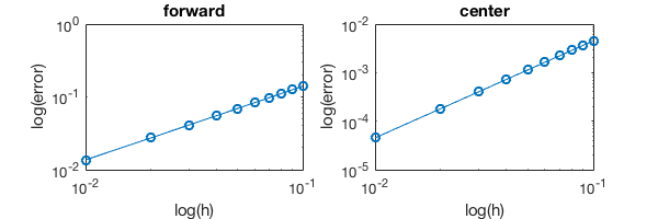
subplot(121); loglog(h_list, error_forward,'-o')
title('forward');xlabel('log(h)');ylabel('log(error)')
subplot(122); loglog(h_list, error_center,'-o')
title('center');xlabel('log(h)');ylabel('log(error)')

To figure out the slope we can do linear regression. You can solve a least square problem as in HW4&5, but here we use a shortcut as described in this example. polyfit(x, y, 1) returns the slope and intercept.

polyfit(log(h_list), log(error_forward), 1)

ans =
    1.0132    0.3662

polyfit(log(h_list), log(error_center), 1)

ans =
    2.0002   -0.7909

The slopes are 1 and 2, respectively. So we’ve verified that forward-diff is 1st-order accurate while center-diff is 2nd-order accurate.

If the analytical solution is not known, you can use the most accurate solution (with the smallest h) as the true solution to figure out the slope. If your numerical scheme is converging to the true solution, then the estimate of order will still be OK. The risk is your numerical scheme might be converging to a wrong solution, and in this case it makes no sense to talk about error convergence.

\(h\) needs to be small

\(error(h) \approx C \cdot h^k\) only holds for small \(h\). When \(h\) is sufficiently small, we say that it is in the asymptotic regime. All the error analysis only holds in the asymptotic regime, and makes little sense when \(h\) is very large.

Let’s make the step size 100 times larger and see what happens.

h_list = 1:1:10; % h is 100x larger than before

% -- the codes below are exactly the same as before --

n = length(h_list);
g_forward = zeros(1,n); % to hold forward difference results
g_center = zeros(1,n); % to hold center difference results

for i = 1:n % loop over different step sizes
    h = h_list(i); % get step size

    % forward difference
    g_forward(i) = (f(x0+h) - f(x0))/h;

    % center difference
    g_center(i) = (f(x0+h) - f(x0-h))/(2*h);
end

error_forward = abs(g_forward - g_true);
error_center = abs(g_center - g_true);

%plot -s 600,200
subplot(121); loglog(h_list, error_forward,'-o')
title('forward');xlabel('log(h)');ylabel('log(error)')
subplot(122); loglog(h_list, error_center,'-o')
title('center');xlabel('log(h)');ylabel('log(error)')

Now the error is super large and the log-log plot is not a straight line. So keep in mind that for most numerical schemes we always assume small \(h\).

So how small is “small”? It depends on the scale of your problem and how rapidly \(f(x)\) changes. If the problem is defined in \(x \in [0,0.001]\), then \(h=0.001\) is not small at all!

Error convergence of numerical intergration

Now consider

\[I = \int_0^1 f(x)\]

We still use \(f(x) = e^x\) for convenience, as the integral of \(e^x\) is still \(e^x\).

f = @(x) exp(x); % the function we want to integrate

I_true = exp(1)-exp(0)

I_true =
    1.7183

We use composite midpoint scheme to approximate \(I\). We test different interval size \(h\). Note that we need to first define the number of intervals \(m\), and then get the corresponding \(h\), because \(m\) has to be an integer.

m_list = 10:10:100; % number of points
h_list = 1./m_list; % interval size

n = length(m_list);
I_list = zeros(1,n); % to hold intergration results

for i=1:n % loop over different interval sizes (or number of intevals)
    m = m_list(i);
    h = h_list(i);

    % get edge points
    x_edge = linspace(0, 1, m+1);

    % edge to middle
    x_mid = (x_edge(1:end-1) + x_edge(2:end))/2;

    % composite midpoint intergration scheme
    I_list(i) = h*sum(f(x_mid));
end

The result is quite accurate.

I_list

I_list =
  Columns 1 through 7
    1.7176    1.7181    1.7182    1.7182    1.7183    1.7183    1.7183
  Columns 8 through 10
    1.7183    1.7183    1.7183

The error is at the order of \(10^{-3}\).

error_I = abs(I_list-I_true)

error_I =
   1.0e-03 *
  Columns 1 through 7
    0.7157    0.1790    0.0795    0.0447    0.0286    0.0199    0.0146
  Columns 8 through 10
    0.0112    0.0088    0.0072

Again, a log-log plot will provide more insights about the order of convergence.

%plot -s 600,200
subplot(121);plot(h_list, error_I, '-o')
title('error -- h');xlabel('h');ylabel('error')
subplot(122);loglog(h_list, error_I, '-o')
title('log(error) -- log(h)');xlabel('log(h)');ylabel('log(error)')

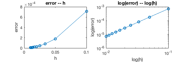
The slope is 2, so the method is second order accurate.

polyfit(log(h_list), log(error_I), 1)

ans =
    1.9999   -2.6372

We’ve just applied the same error analysis method on both differentiation and integration. The same method also applies to ODE solving.

Error convergence of ODE solving

Consider a simple ODE

\[\frac{dy(t)}{dt} = y(t),\ \ y(0)=1\]

The exact solution is \(y(t) = e^t\). We use the forward Euler scheme to solve it.

\[\frac{y(t+h) - y(t)}{h} \approx y(t)\]

The iteration is given by

\[y(t+h) = y(t) + h \cdot y(t) = (1+h)y(t)\]

Let’s only consider \(t \in [0,1]\). More specifically, we’ll only look at the final state \(y(1)\), so we don’t need to record every step.

y1_true = exp(1) % true y(1)

y1_true =
    2.7183

Same as in the integration section, we need to first define the number of total iterations \(m\), and then get the corresponding step size \(h\). This ensures we will land exactly at \(t=1\), not its neighbours.

y0 = 1; % initial condition

m_list = 10:10:100; % number of iterations to get to t=1
h_list = 1./m_list; % step size

n = length(m_list);
y1_list = zeros(1,n); % to hold the final point

for i=1:n % loop over different step sizes
    m = m_list(i); % get the number of iterations
    h = h_list(i); % get step size

    y1 = y0; % start with y(0)

    % Euler scheme begins here
    for t=1:m
        y1 = (1+h)*y1; % no need to record intermediate results here
    end

    y1_list(i) = y1; % only record the final point

end

As \(h\) shrinks, our simulated \(y(1)\) gets closer to the true result.

y1_list

y1_list =
  Columns 1 through 7
    2.5937    2.6533    2.6743    2.6851    2.6916    2.6960    2.6991
  Columns 8 through 10
    2.7015    2.7033    2.7048

error_y1 = abs(y1_list-y1_true)

error_y1 =
  Columns 1 through 7
    0.1245    0.0650    0.0440    0.0332    0.0267    0.0223    0.0192
  Columns 8 through 10
    0.0168    0.0149    0.0135

\(error \leftrightarrow h\) plot is a straight line, so we know the method is fist order accurate. The log-log plot is not quite necessary here.

%plot -s 600,200
subplot(121);plot(h_list, error_y1, '-o')
title('error -- h');xlabel('h');ylabel('error')
subplot(122);loglog(h_list, error_y1, '-o')
title('log(error) -- log(h)');xlabel('log(h)');ylabel('log(error)')

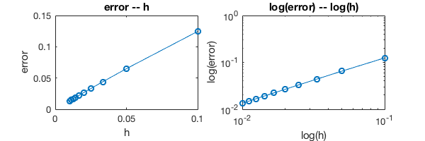
Of course we can still calculate the slope of the log-log plot, to double check the forward Euler scheme is a first-order method.

polyfit(log(h_list), log(error_y1), 1)

ans =
    0.9687    0.1613

The take-away is, you can think about the order of a method in a more general sense. We’ve covered numerical differentiation, intergration and ODE here, and similar analysis also applies to root-finding, PDE, optimization, etc…