Session 10: Fast Fourier Transform

Date: 11/27/2017, Monday

format compact

Generate input signal

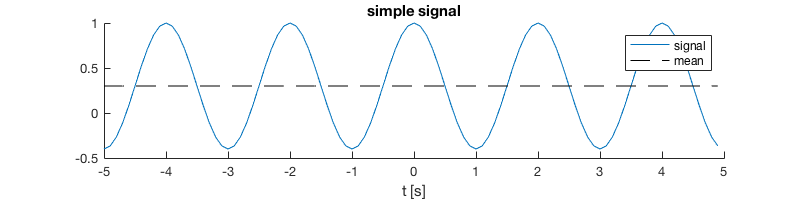
Fourier transform is widely used in signal processing. Let’s looks at the simplest cosine signal first.

Define

\[y_1(t) = 0.3 + 0.7\cos(2\pi f_1t)\]

It has a magnitude of 0.7, with a constant bias term 0.3. We choose the frequency \(f_1=0.5\).

t = -5:0.1:4.9; % time axis
N = length(t) % size of the signal

f1 = 0.5; % signal frequency
y1 = 0.3 + 0.7*cos(2*pi*f1*t); % the signal

N =
   100

%plot -s 800,200
hold on
plot(t, y1)
plot(t, 0.3*ones(N,1), '--k')
title('simple signal')
xlabel('t [s]')
legend('signal', 'mean')

Perform Fourier transform on the signal

You can hand code the Fourier matrix as in the class, but here we use the built-in function for convenience.

F1 = fft(y1);
length(F1) % same as the length of the signal

ans =
   100

There are two different conventions for the normalization factor in the Fourier matrix. One is having the normalization factor \(\frac{1}{\sqrt{N}}\) in the both the Fourier matrix \(A\) and the inverse transform matrix \(B\)

\[\begin{split}A = \frac{1}{\sqrt{N}} \begin{bmatrix} 1&1&1&\cdots &1 \\ 1&\omega&\omega^2&\cdots&\omega^{N-1} \\ 1&\omega^2&\omega^4&\cdots&\omega^{2(N-1)}\\ \vdots&\vdots&\vdots&\ddots&\vdots\\ 1&\omega^{N-1}&\omega^{2(N-1)}&\cdots&\omega^{(N-1)(N-1)}\\ \end{bmatrix}\end{split}\]

\[\begin{split}B = \frac{1}{\sqrt{N}} \begin{bmatrix} 1&1&1&\cdots &1 \\ 1&\omega^{-1}&\omega^{-2}&\cdots&\omega^{-(N-1)} \\ 1&\omega^{-2}&\omega^{-4}&\cdots&\omega^{-2(N-1)}\\ \vdots&\vdots&\vdots&\ddots&\vdots\\ 1&\omega^{-(N-1)}&\omega^{-2(N-1)}&\cdots&\omega^{-(N-1)(N-1)}\\ \end{bmatrix}\end{split}\]

MATLAB uses a different convention that

\[\begin{split}A = \begin{bmatrix} 1&1&1&\cdots &1 \\ 1&\omega&\omega^2&\cdots&\omega^{N-1} \\ 1&\omega^2&\omega^4&\cdots&\omega^{2(N-1)}\\ \vdots&\vdots&\vdots&\ddots&\vdots\\ 1&\omega^{N-1}&\omega^{2(N-1)}&\cdots&\omega^{(N-1)(N-1)}\\ \end{bmatrix}\end{split}\]

\[\begin{split}B = \frac{1}{N} \begin{bmatrix} 1&1&1&\cdots &1 \\ 1&\omega^{-1}&\omega^{-2}&\cdots&\omega^{-(N-1)} \\ 1&\omega^{-2}&\omega^{-4}&\cdots&\omega^{-2(N-1)}\\ \vdots&\vdots&\vdots&\ddots&\vdots\\ 1&\omega^{-(N-1)}&\omega^{-2(N-1)}&\cdots&\omega^{-(N-1)(N-1)}\\ \end{bmatrix}\end{split}\]

The difference doesn’t matter too much as long as you use one of them consistently. In both cases there is

\begin{align} F &= AY \text{ (Discrete Fourier transfrom)} \\ Y &= BF \text{ (Inverse transfrom)} \end{align}

Full spectrum

The spectrum F1 (the result of the Fourier transfrom) is typically an array of complex numbers. To plot it we need to use absolute magnitude.

%plot -s 800,200
plot(abs(F1),'- .')
title('unnormalized full spectrum')

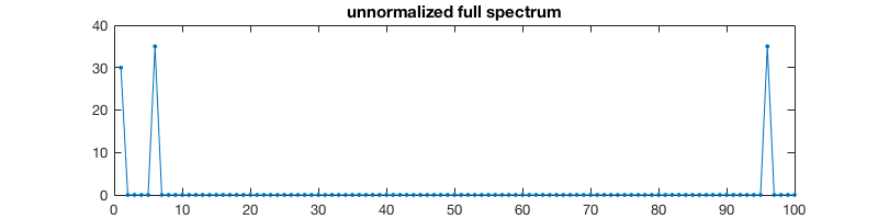
The first term in F1 indicates the magnitude of the constant term (zero frequency). Diving by N gives us the actual value.

F1(1)/N % equal to the constant bias term specified at the beginning

ans =
    0.3000

Besides the constant bias F1(1), there are two non-zero pointings in F1, indicating the cosine signal itself. The magnitude 0.7 is evenly distributed to two points.

F1(2+4)/N, F1(end-4)/N % adding up to 0.7

ans =
  -0.3500 - 0.0000i
ans =
  -0.3500 + 0.0000i

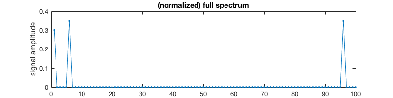
Plotting F1/N shows more clearly the magnitude of signals at different frequencies:

%plot -s 800,200
plot(abs(F1)/N,'- .')
title('(normalized) full spectrum')
ylabel('signal amplitude')

Half-sided spectrum

From the matrix \(A\) it is easy to show that, the first element F(1) in the resulting spectrum is always a real number indicating the constant bias term, while the rest of the array F(2:end) is symmetric, i.e. F(2) == F(end), F(3) == F(end-1). ( F(2) is actually the conjugate of F(end), but we only care about magnitude here. )

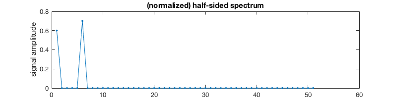
Due to such symmetricity, we can simply plot half of the array (scaled by 2) without loss of information.

M = N/2 % need to cast to integer if N is an odd number

M =
    50

%plot -s 800,200
plot(abs(F1(1:M+1))/N*2, '- .')
title('(normalized) half-sided spectrum')
ylabel('signal amplitude')

Understanding units!

The Discrete Fourier Transform, by defintion, is simply a matrix multiplication which acts on pure numbers. But real physical signals have units. You cannot just treat the resulting array F1 as some unitless frequency. If the signal is a time series then you need to deal with seconds and hertz; if it is a wave in the space then you need to deal with the wave length in meters.

In order to understand the unit of the resulting spectrum F1, let’s look at the original time series y1 first.

The “time step” of the signal is

dt = t(2)-t(1) % [s]

dt =
    0.1000

This is the finest temporal resolution the signal can have. It corresponds the highest frequency:

f_max = 1/dt % [Hz]

f_max =
   10.0000

On the contrary, the longest time range (dt*N, the time span of the entire signal) corresponds to the lowest frequency:

df = f_max/N % [Hz]

df =
    0.1000

With the lowest frequency df being the “step size” in the frequency axis, the value of the frequency axis is simply the array [0, df, 2*df, …]. Now we can use correct values and units for the x-axis of the spectrum plot.

%plot -s 800,200
plot(df*(0:M), abs(F1(1:M+1))/N*2,'- .')
title('half-sided spectrum with correct unit of x-axis')
ylabel('signal amplitude')
xlabel('frequency [Hz]')

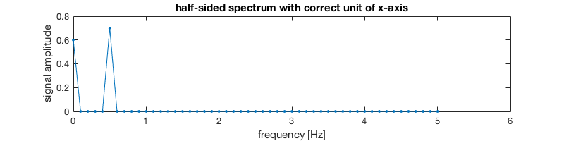
The peak is at 0.5 Hz, consistent with our original signal which has a period of 2 s, since 0.5 Hz = 1/(2s). Thus our unit specification is correct.

Deal with negative frequency

The right half of the spectrum array (F1(M+2:end), not plotted in the above figure) corresponds to negative frequency [-M*df, …, -2*df, -df]. Thus each element in the entire F1 array corresponds to each element in the frequency array [0, df, 2*df, …, M*df, -M*df, …, -2*df, -df].

You can perform fftshift on the resulting spectrum F1 to swap its left and right parts, so it will align with the motonically increasing axis [-M*df, …, -2*df, -df, 0, df, 2*df, …, M*df]. That feels more natural from a mathematical point of view.

F_shifted = fftshift(F1);
plot(abs(F_shifted),'- .')

Perform inverse transform

Performing inverse transform is simply ifft(F1). Recall that MATLAB performs the \(\frac{1}{N}\) scaling during the inverse transform step.

We use norm to check if ifft(F1) is close enough to y1.

norm(ifft(F1) - y1) % almost zero

ans =
   1.2269e-15

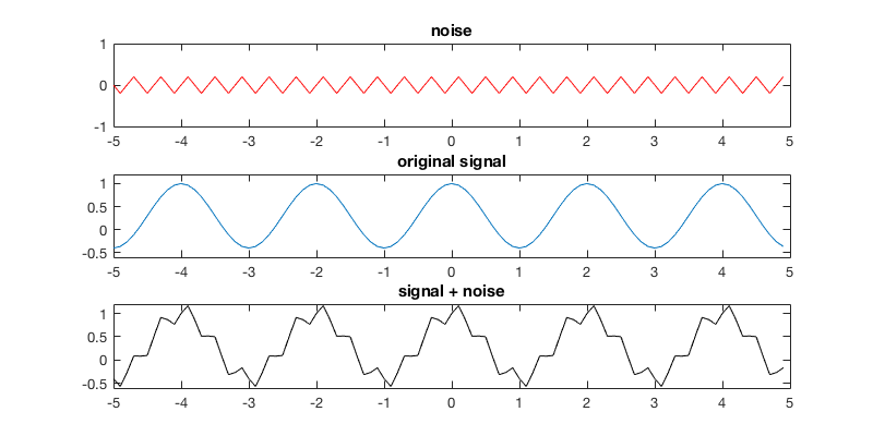
Mix two signals

Fourier transform and inverse transform are very useful in signal filering. Let’s first add a high-frequency noise to our original signal.

f2 = 5; % higher frequency
y2 = 0.2*sin(f2*pi*t); % noise
y = y1 + y2; % add up original signal and noise

%plot -s 800,400
subplot(311);plot(t, y2, 'r');
ylim([-1,1]);title('noise')

subplot(312);plot(t, y1);
ylim([-0.6,1.2]);title('original signal')

subplot(313);plot(t, y, 'k');
ylim([-0.6,1.2]);title('signal + noise')

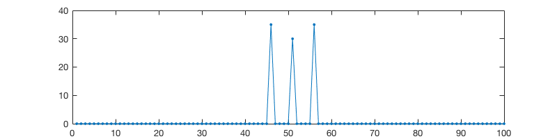
After the Fourier transform, we see two new peaks at a relatively higher frequency.

F = fft(y);

%plot -s 800,200
plot(abs(F), '- .')
title('spectrum with high-frequency noise')

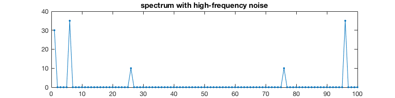
Again, the noise magnitude 0.2 is evenly distributed to positive and negative frequencies. Here we got complex conjugates:

F(2+24)/N, F(end-24)/N % magnitude of noises

ans =
  -0.0000 + 0.1000i
ans =
  -0.0000 - 0.1000i

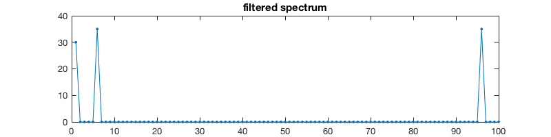
Filter out high-frequency noise

Let’s wipe out this annoying noise. It’s very difficult to do so in the original signal, but very easy to do in the spectrum.

F_filtered = F; % make a copy
F_filtered(26) = 0; % remove the high-frequency noise
F_filtered(76) = 0; % same for negative frequency

plot(abs(F_filtered), '- .')
title('filtered spectrum')

Then we can transform the spectrum back to the signal.

y_filtered = ifft(F_filtered);

If the filtering is done symmetrically (i.e. do the same thing for positive and negative frequencies), the recovered signal will only contain real numbers.

%plot -s 800,200
plot(t, y_filtered)
title('de-noised signal')

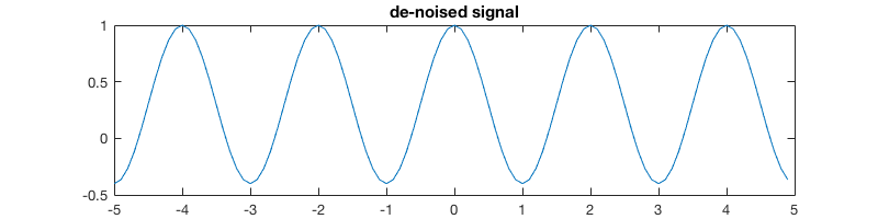
The de-noised signal is almost the same as the original noise-free signal:

norm(y_filtered - y1) % almost zero

ans =
   5.6847e-15

Filter has to be symmetric

What happens if the filtering done asymmetrically?

F_wrong_filtered = F; % make another copy
F_wrong_filtered(76) = 0; % only do negative frequency

plot(abs(F_wrong_filtered), '- .')
title('asymmetrically-filtered spectrum')

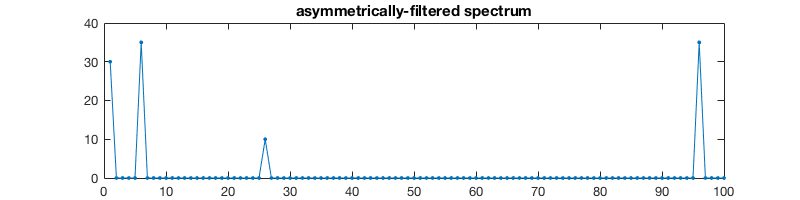
The recovered signal now contains imaginary parts. That’s unphysical!

y_wrong_filtered = ifft(F_wrong_filtered);

y_wrong_filtered(1:5)' % print the first several elements

ans =
  -0.4000 - 0.1000i
  -0.4657 + 0.0000i
  -0.2663 + 0.1000i
  -0.0114 - 0.0000i
   0.0837 - 0.1000i

norm(imag(y_wrong_filtered)) % not zero

ans =
    0.7071

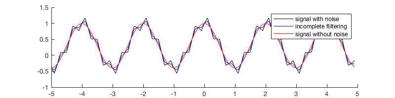
You can plot the real part only. It is something between the unfiltered and filtered signals, i.e. the filtering here is incomplete.

hold on
plot(t, y, 'k')
plot(t, real(y_wrong_filtered), 'b')
plot(t, y1, 'r')
legend('signal with noise', 'incomplete fliltering', 'signal without noise')